Transformation is required to achieve homoscedasticity when we
perform ANOVA to test the effect of factors on the population abundance. The
effectiveness of transformations decreases when data contain zeros. Especially,
the logarithmic
transformation or the Box-Cox transformation is not applicable in such a case.
For the logarithmic transformation, 1 is traditionally added to avoid such
problems.
However, there is no concrete foundation of why 1 is added rather than other
constants, such as 0.5 or 2, although the result of ANOVA is much influenced
by the added
constant. In this paper, I suggest that 0.5 is preferable to 1 as an added constant,
because a discrete distribution defined in {0,1,2,...} is approximately described
by a corresponding continuous distribution defined in (0, infinity) if we add
0.5. Numerical investigation confirms this prediction. (Copyright by the Society
of Population Ecology and Springer-Verlag Tokyo)
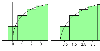 |
Figure 1. Approximation
of a discrete distribution defined in {0, 1. 2, ..} by a continuous
distribution defined in(0,infinity).
(Left panel) Insufficient approximation without adding constant. (Right
panel) Improved approximation by adding 0.5. (Copyright by the Society
of Population Ecology and Springer-Verlag Tokyo)
|
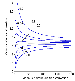 |
Figure 2. Effects of adding
constant (c) on the stabilization of variance of a negative binomial
distribution with a constraint s2 = m2.
A logarithmic transformation, loge(x + c),
is used. Each number beside a solid curve indicates the c used
in the calculation. The dotted curve is that of a gamma distribution(which
is a continuous distribution corresponding to a negative binomial distribution)
with the same constraint for variance. The curve for c = 0.5
is more horizontal than that for c = 1. Therefore, c =
0.5 is superior in achieving homoscedasticity that is required to perform
correct ANOVA. Although most of statistical textbooks recommend the
transformation loge(x + 1), it is a bad custom.
(Copyright by the Society of Population Ecology and Springer-Verlag
Tokyo)
|
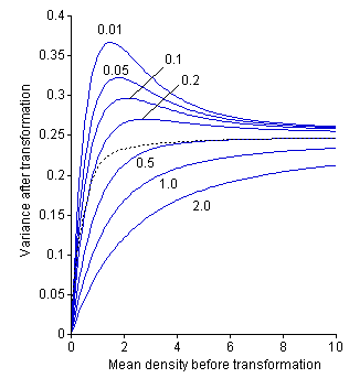 |
Figure 3. Effects of adding constant
(c) on the stabilization of variance of a negative binomial
distribution with a constraint s2 = m. A
square root transformation, sqrt(x + c), is used. Meaning
of each curve is the same as Fig. 2. This case has been discussed
by Bartlett (1936). The variance after transformation for c = 0.5 quickly converges to that of a gamma distribution with increasing
mean. (Copyright by the Society
of Population Ecology and Springer-Verlag Tokyo)
|
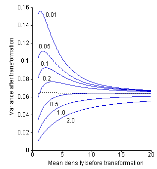 |
Figure 4. Effects of adding
constant (c) on the stabilization of variance of a negative binomial
distribution with a constraint s2 = m1.5.
A power transformation, (x + c)0.25, is used.
Meaning of each curve is the same as Fig. 2. (Copyright by the Society
of Population Ecology and Springer-Verlag Tokyo)
|
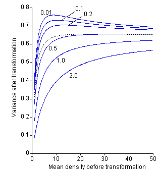 |
Figure 5. Effects of adding
constant (c) on the stabilization of variance of a negative binomial
distribution with a constraint s2 = 0.5(m + m2). An arc-hyperbolic transformation, loge(sqrt(x + c) + sqrt(x + c + 1)), is used. Meaning of each
curve is the same as Fig. 2. (Copyright by the Society of Population
Ecology and Springer-Verlag Tokyo)
|