(1) Analysis of abundance
Table 1. Life table of the beet semi-looper Autographa nigrisigna to illustrate the usefulness of key-factor/key-stage analysis. s0 indicates the natural logarithm of the number of individuals of the 1st stage larvae. si (i = 1, 2, 3) indicate the natural logarithm of survival rate of the i th stage larvae. loge(N4) indicates the natural logarithm of the number of individuals of the 4th instar larvae.
Experiment number |
Experimental block |
Plant density |
s0 |
s1 |
s2 |
s3 |
loge(N4) |
1 |
1 |
sparse |
3.0375 |
-0.6876 |
-0.5116 |
-0.8171 |
1.0212 |
2 |
2 |
sparse |
3.1587 |
-1.0309 |
-0.7252 |
-0.8148 |
0.5878 |
3 |
3 |
sparse |
3.2480 |
-0.9627 |
-0.6292 |
-0.6503 |
1.0059 |
4 |
4 |
sparse |
2.9592 |
-0.6798 |
-0.6759 |
-1.2202 |
0.3833 |
5 |
1 |
dense |
2.4684 |
-0.7314 |
-0.5615 |
-0.4142 |
0.7613 |
6 |
2 |
dense |
2.3188 |
-0.8368 |
-0.3829 |
-0.6250 |
0.4741 |
7 |
3 |
dense |
2.3946 |
-0.6550 |
-0.4126 |
-0.4743 |
0.8527 |
8 |
4 |
dense |
2.8446 |
-0.8896 |
-0.5469 |
-0.2750 |
1.1330 |
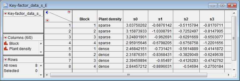
Figure 1. Data table for JMP.
Double click the column title 'Block' to modify the property of variable. Set 'Modelling type' nominal.
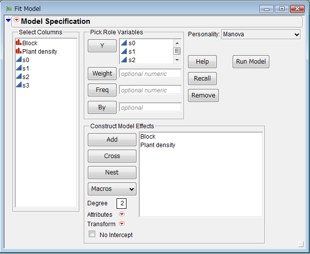
Figure 2. The above dialog box appears when we select 'Fit Model' from 'Analyze' menu of the menu bar. Select s0, s1, s2, s3 from 'Select Columns' box and drag them into 'Y' box. Select 'Block' and 'Plant density' from 'Select Columns' box and drag them into 'Construct Model Effects' box. Select the 'Manova' from the 'Personality' pull down menu in the dialog box. Then, perform analysis by pushing 'Run Model' button.
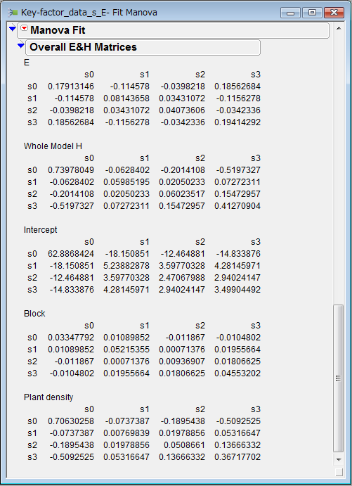
Figure 3. Open the 'Overall E&H Matrices' in the result window. (This matrix is folded in the first view.) Add the s0 row of 'Block' matrix. Then, we obtain 0.03347792 + 0.01089852 + 0.011867 - 0.0104802 = 0.02202924. This quantity indicates the amount of contribution of 'Block' through the abundance in the first stage (s0). Add the s1 row of 'Block' matrix. Then, we obtain 0.01089852 + 0.05215355 + 0.00071376 + 0.01955664 = 0.08332247. This quantity indicates the amount of contribution of 'Block' through the survival rate in the first stage (s1). Perform the similar calculation for each row of the following three matrices: Block, Plant density, and E. Then, we obtain the key-factor/key-stage analysis table by arranging the calculated 12 quantities.
Table 2. Key-factor/key-stage table. Components are multiplied by 10000 to facilitate the mutual comparison.
Factor |
df |
Stage |
Total |
|||
s0 |
s1 |
s2 |
s3 |
|||
Block |
3 |
220.3 |
833.2 |
162.8 |
726.7 |
1943.1 |
Plant density |
1 |
-662.3 |
69.1 |
177.7 |
477.5 |
62.1 |
Residual |
3 |
2103.6 |
-1144.6 |
9.9 |
2299.1 |
3268.0 |
Total |
7 |
1661.6 |
-242.2 |
350.5 |
3503.4 |
5273.2 |
Example analysis using JMP
(2) Analysis of mortality
Table 3. Life table of the beet semi-looper Autographa nigrisigna to illustrate the usefulness of key-factor/key-stage analysis. ki (i = 1, 2, 3) indicate the negative natural logarithm of survival rate of the i th stage larvae.
Experiment number |
Experimental block |
Plant density |
k1 |
k2 |
k3 |
K |
1 |
1 |
sparse |
0.2986 |
0.2222 |
0.3548 |
0.8757 |
2 |
2 |
sparse |
0.4477 |
0.3150 |
0.3539 |
1.1165 |
3 |
3 |
sparse |
0.4181 |
0.2732 |
0.2824 |
0.9738 |
4 |
4 |
sparse |
0.2952 |
0.2935 |
0.5299 |
1.1187 |
5 |
1 |
dense |
0.3177 |
0.2439 |
0.1799 |
0.7414 |
6 |
2 |
dense |
0.3634 |
0.1663 |
0.2714 |
0.8011 |
7 |
3 |
dense |
0.2844 |
0.1792 |
0.2060 |
0.6696 |
8 |
4 |
dense |
0.3863 |
0.2375 |
0.1194 |
0.7433 |
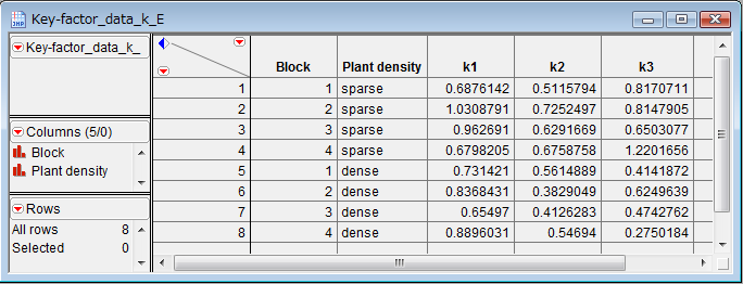
Figure 4. Data table for JMP.
Double click the column title 'Block' to modify the property of variable. Set 'Modelling type' nominal.
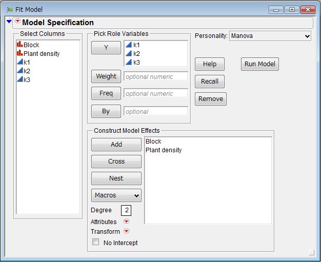
Figure 5. The above dialog box appears when we select 'Fit Model' from 'Analyze' menu of the menu bar. Select k1, k2, k3 from 'Select Columns' box and drag them into 'Y' box. Select 'Block' and 'Plant density' from 'Select Columns' box and drag them into 'Construct Model Effects' box. Select the 'Manova' from the 'Personality' pull down menu in the dialog box. Then, perform analysis by pushing 'Run Model' button.
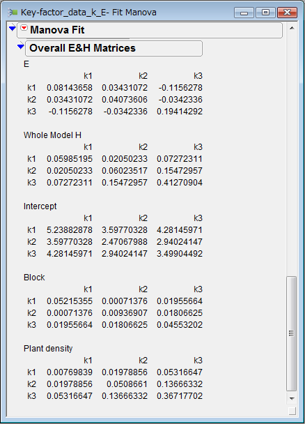
Figure 6. Open the 'Overall E&H Matrices' in the result window. (This matrix is folded in the first view.) Add the k1 row of 'Block' matrix. Then, we obtain 0.05215355 + 0.00071376 + 0.01955664 = 0.07242395 . This quantity indicates the amount of contribution of 'Block' through the survival rate in the first stage (k1). Perform the similar calculation for each row of the following three matrices: Block, Plant density, and E. Then, we obtain the key-factor/key-stage analysis table by arranging the calculated 9 quantities.
Table 4. Key-factor/key-stage table. Components are multiplied by 10000 to facilitate the mutual comparison.
Factor |
df |
Stage |
Total |
||
k1 |
k2 |
k3 |
|||
Block |
3 |
724.2 |
281.5 |
831.5 |
1837.3 |
Plant density |
1 |
806.5 |
2073.2 |
5570.1 |
8449.8 |
Residual |
3 |
1.2 |
408.1 |
442.8 |
852.1 |
Total |
7 |
1532.0 |
2762.8 |
6844.4 |
11139.2 |
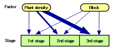
Figure 7. Illustration of the result of key-factor/key-stage analysis . Thickness of arrows is proportional to the corresponding component in Table 2. The arrow that connects the plant density and 3rd stage larvae is extremely thick. Therefore, it is indicated that the number of the 4th stage larvae is principally determined by the plant density through the survival rate of the 3rd stage larvae.